A sketchy surgery description of the Seifert-Weber Dodecahedral space

Gates Rudd, Dunfield, and Obeidin just put out their preprint Computing a link diagram from its exterior. It describes “the first practical algorithm for finding a diagram of a knot given a triangulation of its exterior”. Neat. Really neat. I’ve been doing it the hard way.

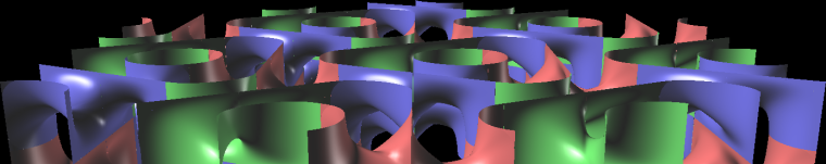
As one application of their work, they found a surgery diagram of the Seifert-Weber Dodecahedral space. Here’s Figure 21 of Section 9.2.

Surgery description of the Seifert Weber space by Gates Rudd, Dunfield, and Obeidin

Here’s one I came up with back in September 2019 in response to a MathOverflow question but never got around to cleaning up for public consumption.

A sketchy surgery description of the Seifert Weber space

Below we’ll take a look at some of the sketches that led to this surgery description.

So I’ll just spit these pictures out with a bit of discussion. Aside from giving space between them and taking snapshots, I’ve not done any other drawings or cleanups. For these drawings I used OneNote.

Along the top with the purple is a quotient of the Whitehead link. That doesn’t get used, so ignore it.

The text in the upper corner says:

SWD is a 5 fold cyclic branched cover of the Whitehead link

However there are two such covers according to the generators vs of .

Goal: Find a surgery diagram.

The first steps were based off the discussion on the MathOverflow post. Let’s look closer at the unlinking of the Whitehead link by a surgery on a red curve. The surgery on this red curve is what gets lifted to the main action of the surgery description.

Taking a 5-fold branched cover of the unlink now, we think of slicing open the two components along the disks they bound. This gives us a that we’ll take five copies of and glue together. The branch loci are the equators on each of the boundary spheres. Here we’re keeping track of how the red curve gets split, and how its ends glue together. Notice that we are using the generator of .

The blue cylinder divides this into two plugs which the branch loci meets in a diameter of each end disk. One side is disjoint from the red arcs, the other side contains the red arcs. The point here is now that in the 5-fold branched cover of the unlink, this cylinder pieces together to give a genus 4 Heegaard surface. Indeed, for each plug, 5 copies piece together around the 2 arcs of branch locus to form a handlebody. The two handlebodies are glued together by a mirroring, so we just need to mind how the plug with the red arcs fits together to form a handlebody with red curves. The lower right shows a flattening of the plug with red arcs to get a better diagrammatic grasp on it for the handlebody assembly.

Forming the handlebody that contains the red curves

Some of the labeling shows how I was keeping track of the gluings. This produced the above collection of red curves in a blue genus 4 handlebody. I guess I didn’t add the outer blue curve on the right.

We also need to pay attention to the surgery slope of the original unlinking of the Whitehead link. So the above is repeated and cleaned up with the extra framing info, shown as an auxiliary green push-off. Luck has it that in our diagrammatic picture of the plug, the framing agrees with the blackboard framing!

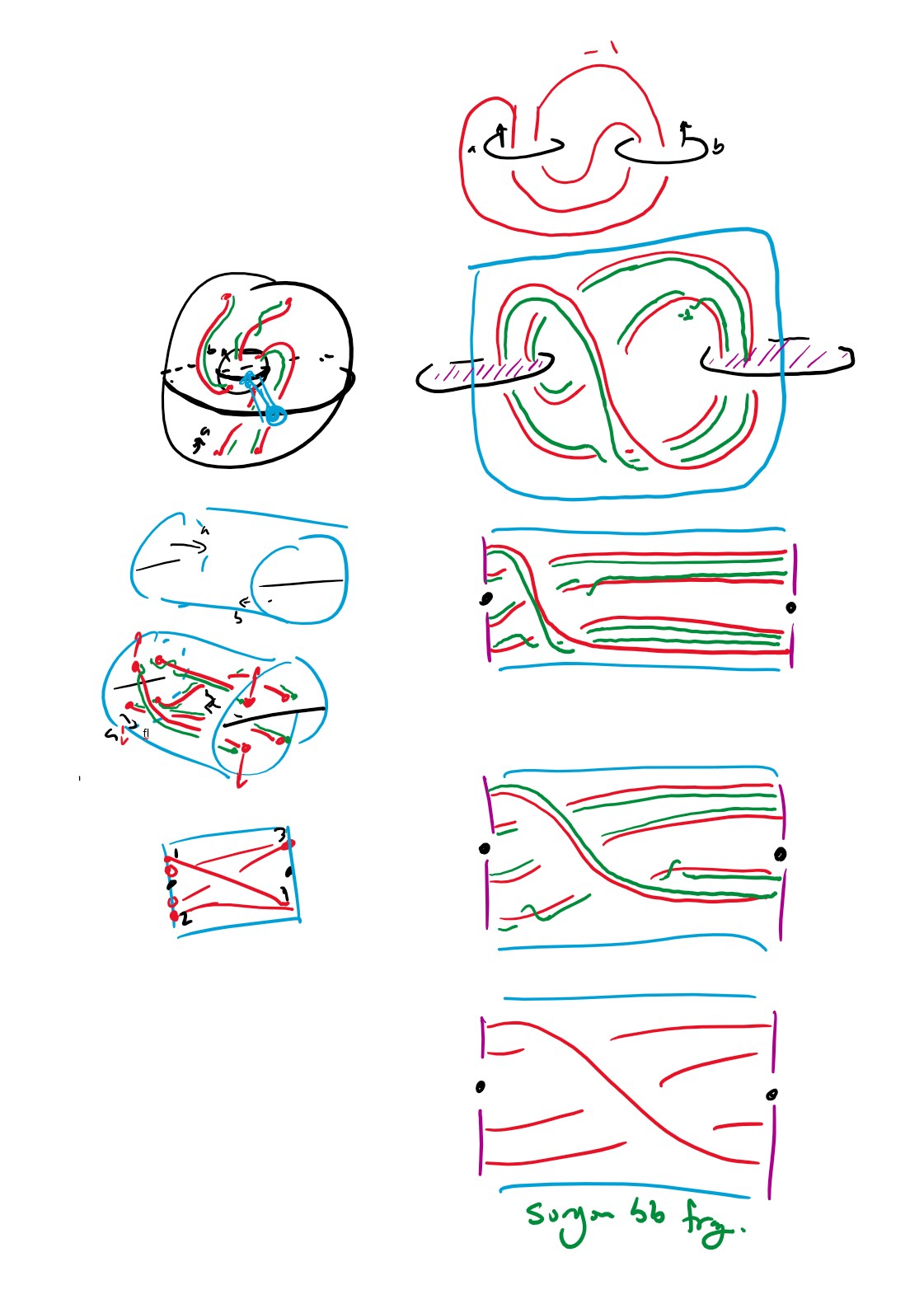
So our earlier picture of the red link in the blue handlebody actually also records the needed framing. This blackboard framing is the writhe of the diagram component. I color coded it to not get the link components mixed up as seen on the right side of the figure below. Then to glue on the empty other handlebody, it suffices to just do 0 surgery on curves that link the 4 handles of the blue handlebody. That gives us the surgery diagram on the right.

As a simple check, I had drawn this link in SnapPy and did surgery on it.

M.dehn_fill([(2,1),(1,1),(-1,1),(-1,1),(0,1),(0,1),(0,1),(0,1),(0,1)])

You can see that SnapPy recognizes this filling as the manifold ododecld01_00007(1,0) which is what it calls the Seifert Weber space. (That last bit got cut off up in this browser window, but the volume and homology should help convince you.)

WordPress doesn’t want me to upload a text file (because it is a danger to you and everyone you love), so below is the contents of the Plink file if you want to try it out. Just past it into a plain text file. Then open it from the Plink menu in SnapPy.

% Link Projection
9
   0    0
  10   10
  17   17
  23   23
  36   36
  80   80
  84   84
  88   88
  92   92
113
  487   240
  471   271
  523   388
  652   393
  843   124
  940   120
  941   262
  811   256
  617    71
   95    85
  297   270
  661   377
  504   373
  399   457
  434   671
 1121   669
 1117   386
 1090   382
 1104   650
  455   653
  435   463
  393   419
  313   363
   79   656
  720   569
  801   465
  960   440
 1005   551
  963   611
  656   525
  666   464
  325   556
  306   468
  370   357
  429   366
  485   449
  442   359
  497   434
  656   511
  950   589
  984   548
  949   466
  805   482
  737   585
   62   676
  235   377
  693   481
  306   579
  300   446
  346   343
  378   252
  502   258
  847   143
  924   144
  927   243
  819   241
  622    56
   76    72
  290   289
  332   221
  313   127
  547   108
  714   294
  439   336
  677   285
  541   128
  332   146
  358   262
  342   280
 1066    80
  803    84
  464   213
  428   294
 1085    69
  797    66
  438   204
  409   291
  350   326
  280   380
  299   344
  345    21
  422    16
  434   176
  367   178
  470    23
  597   263
  541   283
  450    47
  341   522
  371   514
  390   682
  343   675
  523   424
  560   435
  529   696
  490   691
   52   356
   99   222
   78   234
   69   363
  111   623
   89   374
  129   607
  104   380
  170   128
  178   211
  342   201
  203   143
  224   395
  168   537
  285   519
  182   511
  273   505
113
   1    0
   2    1
   3    2
   0    4
   4    5
   5    6
   6    7
   7    8
   8    9
  12   11
  13   12
  14   13
  15   14
  16   15
  18   17
  19   18
  20   19
  21   20
  22   21
  24   23
  25   24
  26   25
  27   26
  28   27
  29   28
  30    3
  31   30
 102   31
  32   33
  33   34
  34   35
  35   29
  37   36
  38   37
  39   38
  40   39
  41   40
  42   41
  43   42
  44   43
  11   46
  46   47
  47  100
  48   49
  50   51
  51   52
  52   53
  53   54
  54   55
  55   56
  56   57
  49   58
  59   50
  60  104
  61   60
  62   61
  36   62
  63   64
  64   65
  65   66
  67  106
  68   67
  17   69
  69   70
  70   71
  71   72
  72   63
  73   16
  74   73
  75   74
  76   75
  77   76
  10   77
  79   68
  45   22
  78   79
  80   81
  81   82
  82   83
  83   80
  84   85
  85   86
  86   87
  87   84
  88   89
  89   90
  90   91
  91   88
  92   93
  93   94
  94   95
  95   92
  96   44
 106   96
   9   97
  57   98
  23   99
 100  101
 101   10
 103  102
  58  103
 104  105
  66  107
 107   45
 105  108
 108   78
  99   59
  98  109
 109  110
 110   32
  97  111
 111  112
 112   48
111
   7    3
   9    1
  17   10
  19   11
  19   16
  20   24
  26   11
  26   16
  28   18
  30   10
  26   31
  32   10
  26   33
  20   34
  38   24
  38   34
  39   11
  39   16
  41   11
  41   16
  41   31
  41   33
  43   18
   0   44
   7   45
  49    3
  49   45
  55    3
  55   45
  56    1
  57    1
  58    3
  58   45
  52   60
   7   64
  49   64
  55   64
  58   64
  65   44
   7   69
  49   69
  55   69
  58   69
  70   44
  51   73
  72   73
  75   74
   8   77
  50   77
  54   77
  59   77
  79    8
  79   50
  79   54
  79   59
   3   80
   8   80
  45   80
  50   80
  54   80
  59   80
  64   80
  69   80
  82    3
  82    8
  82   45
  82   50
  82   54
  82   59
  82   64
  82   69
  19   85
  26   85
  39   85
  41   85
  87   19
  87   26
  87   39
  87   41
  12   89
  15   89
  19   89
  26   89
  31   89
  33   89
  39   89
  41   89
  91   12
  91   15
  91   19
  91   26
  91   31
  91   33
  91   39
  91   41
 103   93
 103   98
 103  100
 104   93
 104   98
 104  100
 103  106
 104  106
 107   93
 107   98
 107  100
 107  106
 110   93
 110   98
 110  100
 110  106
-1

~ by Ken Baker on December 9, 2021.